(un)Adling the First DNA Computer
Addle
(verb) to confuse someone
I use ‘adling’ here as a pun skipping the extra ‘d’ as a tribute to Leonard Adleman who devised the idea for the first DNA computer
Anything Can Be A Computer
When I first started thinking about computing using biomolecules, I had zero idea of how computers actually worked. So I reached out to Y, a geeky senior at college with curly unruffled hair and constantly wearing a black t-shirt with the Maxwell’s equation on it (and an absolute gem of a person) for help.
Y directed me to an intriguing YouTube video by Steve Mould where he attempts to build a ‘water computer’ - directing the flow of water in different ways to develop logic gates (which are devices that take binary inputs and give an output based on an underlying series of instructions called an algorithm). The insight from this video and other similar ones, including logic gates using dominoes, was clear - it doesn’t matter what the physical entity used to build computers is as long as you can create binary conditions within that entity, and facilitate algorithms to carry out desired binary operations.
Identifying a Problem to Solve
This is exactly how Adleman built the first DNA computer in 19941 . He started out by choosing an interesting computational problem to solve - identifying whether an arbitrary directed graph with designated vertices has a Hamiltonian path or not.
If you understand what this means, you can skip the next two paragraphs and move on to looking at the graph. For folks who are unfamiliar with graph theory, I will spend some time breaking down what these words mean, and (hopefully) get you to say, ‘damn, this is actually much easier than it sounds’.
A graph is anything that has vertices and edges - vertices (points representing pieces of data) connected by lines, with the lines indicating the relationship between these points. A directed graph is a graph where the lines (edges) between points (vertices) indicate specific directional relationships, for instance if node A is an input for node B, then the edge between A and B will be an arrow going from A to B. Directed graphs are often used to represent the internet with web pages acting as vertices and hyperlinks between them acting as edges.
A Hamiltonian path is a way to navigate a directed graph in such a manner that it traverses every vertex only once, and does not leave out any vertex. A Hamiltonian path need not be a closed loop, i.e. you don’t need to get back to the starting vertex. If you consider all beaches in Goa to be vertices on the map, land at the MOPA airport in the North, rent out a scooter and go to every single beach until you reach the Dabolim airport in the South you have taken a Hamiltonian path on a directed graph of Goa.
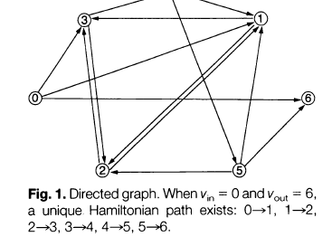
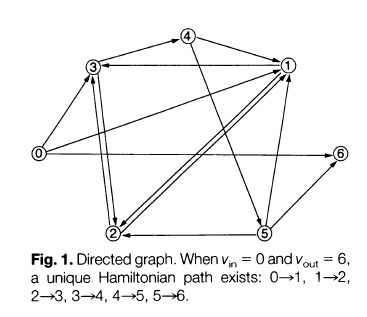
Here is the directed graph that Adleman used for the DNA computer experiment:
The Algorithm
Now that we understand what a Hamiltonian path in a directed graph is, the five-step algorithm used to solve this problem is fairly straightforward:
Generate random paths through the graph, given a particular starting and ending vertex (here the starting vertex is 0 and the ending vertex is 6).
Out of the random paths generated in step 1, keep only those paths that start at vertex 0 and end at vertex 6.
If the graph has ‘n’ nodes, keep only those paths (available after step 2) that enter exactly ‘n’ nodes.
Out of the paths remaining after step 3, keep only those paths that enter all of the vertices of the graph at least once.
If any paths remain, say “yes”. If not, say “no”.
Using DNA to Work the Algorithm
This is where things get interesting because you start with physical experimentation.
Step 1: Generate random paths through the graph
Random 20-nucleotide ( a nucleotide is one of the four bases A, T, C or G that makes up DNA) sequences of DNA were used to denote each of the vertices.
Directed edges (eg: the edge from vertex 1 to 2 in the graph given above) were denoted by using a combination of 10 nucleotides from the 3’ end of the sequence denoting vertex 1 and 10 nucleotides from the 5’ end of the sequence denoting vertex 2. If the edge was directed from vertex 2 to 1, then we would have picked 10 nucleotides from the 3’ end of the sequence denoting vertex 2 and 10 nucleotides from the 5’ end of the sequence denoting vertex 1. If you are unsure of what the 3’ and 5’ ends of the DNA are, you can check out this short video.
Now we need to get these DNA sequences to form random paths. This is done through ligation reactions - a fundamental technique in molecular biology where two compatible DNA fragments are stitched together by an enzyme called ligase. In order to enable ligation, 50 picomoles of the complementary DNA sequences of each vertex (excluding the starting and ending ones) and 50 picomoles of each directed edge were mixed together in a reaction container. This results in a large number of random paths being obtained, at least one out of which is likely to be a Hamiltonian path.
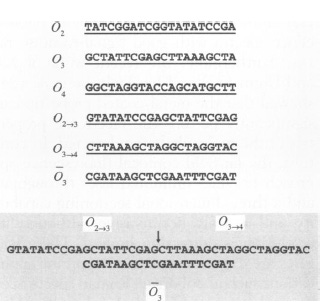
An example of step 1 is as follows:
Here O is used as a term to denote a vertex, O2 indicates vertex 2. O (2 arrow 3) indicates a directed edge from 2 to 3 and O3 with a bar on top indicates the complementary sequence of vertex 3.
Step 2: keep only those paths that start at vertex 0 and end at vertex 6.
The products of step 1 were amplified using a Polymerase Chain Reaction (PCR) with the DNA sequence of vertex 0 and the complementary sequence of vertex 6 as the primers. As a result, only those pathways which start at vertex 0 and end at vertex 6 get amplified. If you are unfamiliar with how PCR works, you can check out this video
Step 3: keep only those paths that enter exactly 7 nodes.
The amplified products from step 2 are loaded on to a gel electrophoresis column, where DNA strands are separated based on weight. The principle is simple - a heavier DNA sequence has slower mobility in the gel as compared to a lighter sequence.
A weight marker (a standard DNA sequence whose size corresponds to the theoretically calculated size of a path that passes through all 7 vertices) is also introduced into a separate lane of the agarose gel matrix to help us identify the sequences that meet this criteria. The DNA from the desired band on the gel matrix were extracted.
Then they carry out a graduated PCR (simultaneously doing PCR in multiple lanes using different primers and temperatures) with the sequence of vertex 0 (SV0) in the first lane and the complementary sequence of vertex 1 (CSV1), 2, 3, 4, 5 and 6 in the corresponding lanes. When gel electrophoresis is done on the PCR products, we get outputs like these:
a) 40, 60, 80, 100, 120, and 140 bp in successive lanes of the electrophoresis if the Hamiltonian path 0→1, 1→2, 2→3, 3→4, 4→5, 5→6 path is followed
b) 40, x, 60, 80, 100, and 120 bp in successive lanes if the 0→1,1→3, 3→4, 4→5, 5→6 path is followed. Here x indicates that there is no band obtained in lane 2 as we skipped vertex 2. This is not a Hamiltonian path.
c) x, 60, 80-40, 100, 120, and140 bp in successive lanes if the 0→3, 3→2, 2→3, 3→4, 4→5, 5→6 path is followed. 80-40 denotes that both a 40-bp and an 80-bp band will be produced in lane 3 because the path traverses vertex 3 twice. This is not a Hamiltonian path either.
(there are many more potential examples of non-Hamiltonian paths, but you get the picture)
Step 4: keep only those paths that enter all of the vertices of the graph at least once.
We are using the brute force method to determine this.
By the end of step 3, we continue to have double stranded DNAs. We now separate these into single stranded DNA molecules (there are multiple ways of doing this including heating, enzymatic treatment, aPCR etc. - but this is not directly relevant to our discussion here so I am skipping the details).
We then incubate these ssDNA molecules with the complementary sequence of vertex 1 (CSV1). CSV1 is attached to a small vitamin-B7 derived molecule called biotin. Biotin has a strong affinity to a naturally occurring protein called avidin. So we use magnetic beads coated with avidin to pull out biotin molecule-attached CSV1s, which would have paired up with the sequence of vertex 1 anyways because of sequence complementarity. This way we are eliminating all path sequences that do not go through vertex 1.
A similar process is repeated with vertices 2-5, and by the end we are left with only those path sequences that go through all vertices.
Step 5: If any paths remain, say “yes”. If not, say “no”.
Another graduated PCR (similar to the one in step 3) is carried out, followed by gel electrophoresis. The most prominent bands in the gel electrophoresis column when viewed under UV illumination shows 40, 60, 80, 100, 120, and 140 bp in successive lanes. This indicates that we have a Hamiltonian path. So yeah, the answer is yes - we have a Hamiltonian path to the given directed graph starting at vertex 0 and ending at vertex. And that path is 0→1, 1→2, 2→3, 3→4, 4→5, 5→6.
This image shows us how we have managed to filter out the DNA sequences of different paths to get to the final answer.
Figure A: Gel electrophoresis after step 2
Figure B: Gel electrophoresis after graduated PCR in step 3
Figure C: Gel electrophoresis in step 5
So we have leveraged DNA as the physical medium to run this algorithm to solve a computational problem. This is what biocomputation looks like at the most primitive level (of course, this was revolutionary in 1994 when it was first introduced).
Room for Error
1. During step 1, ligation mismatches can occur. Non-compatible DNA strands can come together and pass through the other four steps to generate a pseudo-Hamiltonian path. Therefore, we need to identify methods to eliminate ligation mismatches somewhere along the way.
2. As the graph becomes more complex, we would need more DNA sequences to represent vertices and edges, and if we stick to the algorithm used here, the entire process become inefficient in terms of time, as all of the PCR and electrophoresis steps need to be carried out manually (of course, now we have the tools to automate this). The best way to deal with this is to design more efficient algorithms, minimizing the number of steps needed to get to a Hamiltonian path. Adleman’s former grad student Manoj Gopalakrishnan is attempting to build this new class of algorithms at AlgoBio.
What are the Potential Implications of a Computer Like This?
1. Solving Non-Deterministic Polynomial (NP) problems like finding a Hamiltonian path for a directed graph.
An NP problem is any computational decision problem whose solutions are hard to find due to exponential worst-case complexity (which basically means that the time taken to come to a solution increases exponentially for a small linear increase in the size of the dataset).
In this particular experiment we used 50 picomolar concentration of edge sequences, which accounts for nearly 3 X 10^13 sequences. And if a single ligation is taken as a computational operation, we are able to perform nearly 10^14 operations per second, and it can be scaled to 10^20 or more operations by increasing the concentration to micromolar concentrations instead of picomolar. For context, the fastest super computer today can do 1.1 X 10^18 operations per second, which is only 10^6 faster than the fastest supercomputer we had in 1994.
While biocompute maybe slower with respect to ordinary applications like multiplying two integers, the scope of its applications empowers us to do more complex computation.
2. Improving the energy efficiency of compute
1 Joule of energy can potentially power 2 X 10^19 DNA ligation operations, which falls within the current thermodynamic limit of 34 x 10^19 irreversible operations per joule at 300 K (and of course we always push the frontiers of thermodynamic limits through new experiments and use cases). The most efficient super computer today only reaches an efficiency of 10^9 operations per Joule. This shows us how biocompute can make our computing architecture significantly more energy efficient, and hence more sustainable for the planet.
All we have got to do is to design efficient hardware and software to enable DNA (and other biomolecule based) storage and computation, and that’s what we are up to at BioCompute.
“One can imagine the eventual emergence of a general purpose computer consisting of nothing more than a single macromolecule conjugated to a ribosome-like collection of enzymes that act on it” - Leonard Adleman,
Molecular Computations of Solutions to Combinatorial Problems (1994)
I am excited to explore how a ribosome (or a synthetic alternative) can drive compute. That’s probably what the next newsletter will uncover. If you come across interesting resources, please send them my way and let’s catch up and chat about it.
Molecular Computations of Solutions to Combinatorial Problems, published in Science in 1994 (you can use platforms like SciHub to access this paper for free if you are not affiliated with an academic institution)


